School of Mathematics, The University of Edinburgh
Published
July 22, 2018
Updated 2024-01-27 to use the fmesher package. Need fmesher version 0.2.0.9009 or later.
The fmesher package has several features that aren’t widely known. The code started as an implementation of the triangulation method detailed in Hjelle and Dæhlen, “Triangulations and Applications” (2006), which includes methods for spatially varying mesh quality.1 Over time, the interface and feature improvements focused on robustness and calculating useful mesh properties, but the more advanced mesh quality features are still there!
The algorithm first builds a basic mesh, including any points the user specifies, as well as any boundary curves (if no boundary curve is given, a default boundary will be added), connecting all the points into a Delauney triangulation.
After this initial step, mesh quality is decided by two criteria:
Minimum allowed angle in a triangle
Maximum allowed triangle edge length
As long as any triangle does not fulfil the criteria, a new mesh point is added in a way that is guaranteed to locally fix the problem, and a new Delaunay triangulation is obtained. This process is repeated until all triangles fulfil the criteria. In perfect arithmetic, the algorithm is guaranteed to converge as long as the minimum angle criterion is at most 21 degrees, and the maximum edge length criterion is strictly positive.
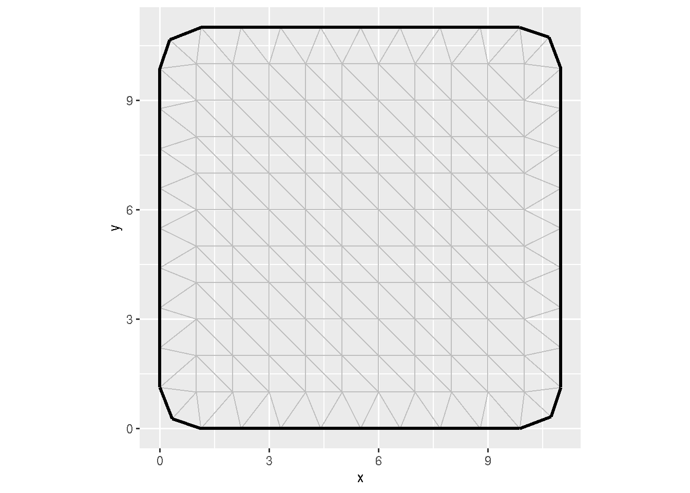
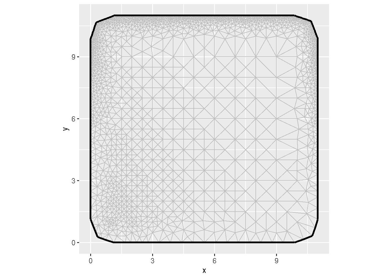
A basic mesh with regular interior triangles can be created as follows:
# See INLA installation instructions on https://www.r-inla.org/download-installlibrary(INLA) # Only needed for inla.mesh.assessment()library(inlabru)library(ggplot2)library(fmesher)loc <-as.matrix(expand.grid(1:10, 1:10))bnd <-fm_nonconvex_hull_inla(loc, convex =1, concave =10)mesh1 <-fm_rcdt_2d_inla(loc = loc,boundary = bnd,refine =list(max.edge =Inf))ggplot() +gg(mesh1) +coord_equal()
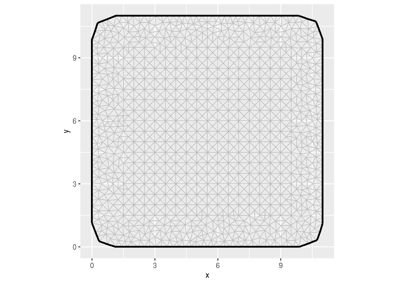
The fm_nonconvex_hull_inla function creates a polygon to be used as the boundary of the mesh, extending the domain by a distance convex from the given points, while keeping the outside curvature radius to at least concave. In this simple example, we used the method fm_rcdt_2d_inla, which is the most direct interface to fmesher. The refine = list(max.edge = Inf) setting makes fmesher enforce the default minimum angle criterion (21 degrees) but ignore the edge length criterion. To get smaller triangles, we change the max.edge value:
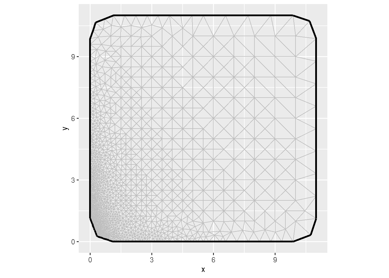
It is often possible and desirable to increase the minimum allowed angle to achieve smooth transitions between small and large triangles (values as high as 26 or 27, but almost never as high as 35, may be possible). Here we will instead focus on the edge length criterion, and make that spatially varying.
We now define a function that computes our desired maximal edge length as a function of location, and feed the output of that to fm_rcdt_2d_inla using the quality.spec parameter instead of max.edge:
We can also make more complicated specifications, but beware of asking only for reasonable triangulations; When experimenting, I recommend setting the max.n.strict and max.n values in the refine parameter list, that prohibits adding infinitely many triangles!
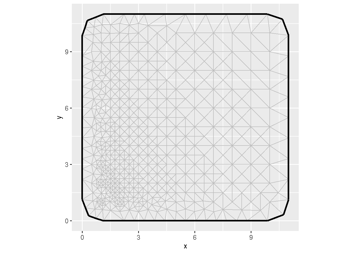
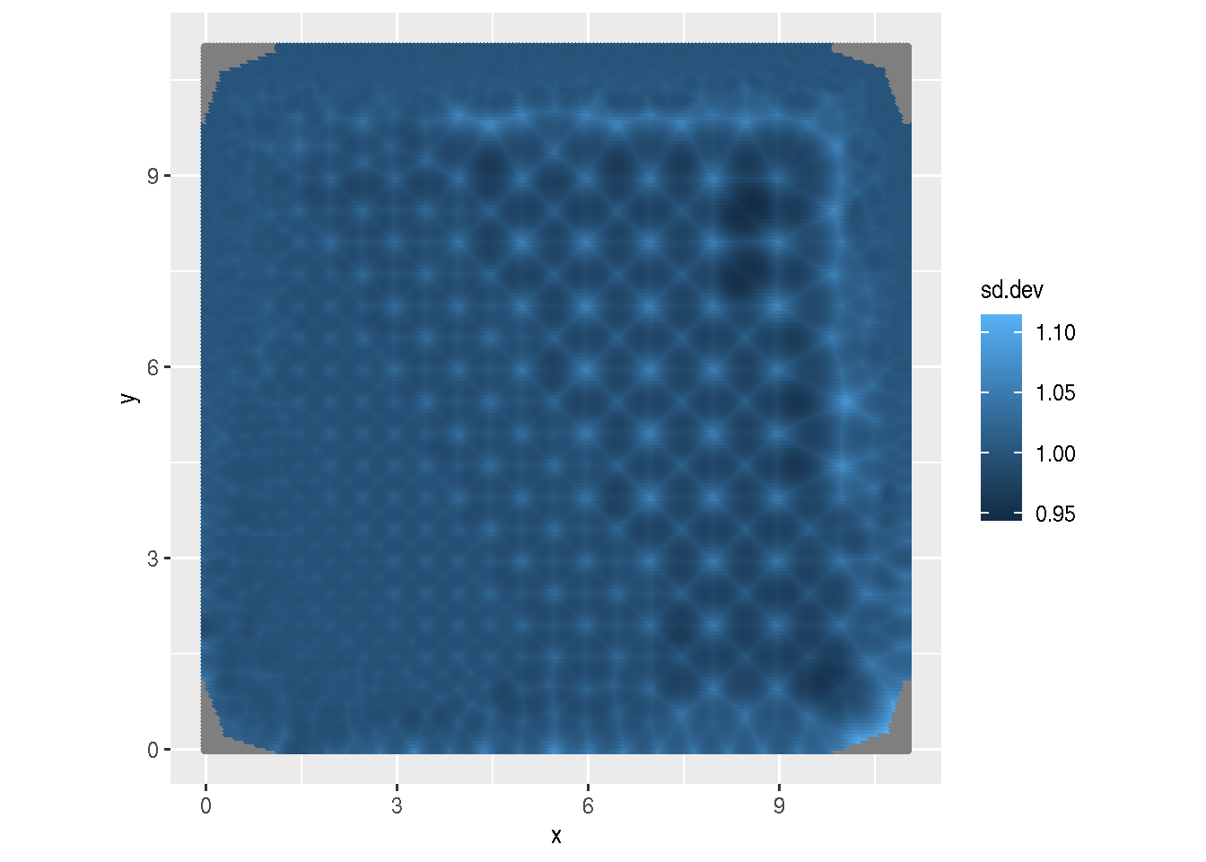
A “good” mesh should have sd.dev close to 1; this indicates that the nominal variance specified by the continuous domain model and the variance of the discretise model are similar.
Here, we see that the standard deviation of the discretised model is smaller in the triangle interiors than at the vertices, but the ratio is close to 1, and more uniform where the triangles are small compared with the spatial correlation length that we set to 5. The most problematic points seem to be in the rapid transition between large and small triangles. We can improve things by increasing the minimum angle criterion:
The algorithm is very similar to the one used by triangle, available in R via Rtriangle. That only handles planar meshes, and has a potentially problematic non-commercial license clause. Since we needed spherical triangulations for global models, we had to write our own implementation.↩︎